Additive and Non-Additive Variables I: Definitions and Properties

When performing an estimation or simulation of a new variable, it is important to ask about its additive property, its linearity, and understand its definition. If the variable is not additive, this knowledge allows us to evaluate appropriate methodologies and techniques for estimating it — for example, by simplifying, referring to its defining equations, or applying domains where the variable behaves approximately linearly.

Understanding the nature of variables allows us to establish their mathematical properties — for instance, to assume linearity — or their geological properties to adopt valid criteria for conceptualising their behaviour (for example, determining that a variable behaves differently under certain geochemical or geophysical conditions). This understanding ultimately allows us to extrapolate values through space and/or time.

But how is an additive variable defined? How can we distinguish an additive variable from a non-additive one? What are their characteristics? How should we approach the estimation of non-additive variables?

Let us begin with the definition and properties of variables to understand and differentiate additive from non-additive ones:

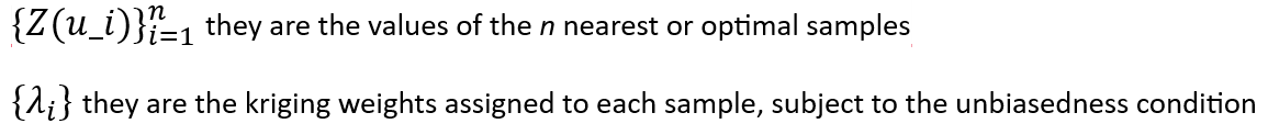
First, an additive variable is one whose total value equals the sum of its parts, such as length (m), area (m²), volume (m³), or tonnage (mass). For example: 2 m³ + 3 m³ = 5 m³.

Second, let us consider the concepts of extensive and intensive properties. A property is extensive when it depends on the size, amount, or extent of the system. These variables are additive, such as mass and volume: if two samples are combined, their extensive properties are summed. For example, if two objects have masses of 2 kg and 3 kg, the total mass will be 5 kg. Conversely, a property is intensive when it does not depend on the size, amount, or extent of the system. Intensive properties — such as density, temperature, and pressure — are not additive when combining systems. For instance, if you have one litre of water with a density of 1 g/cm³ and add another litre with the same density, the resulting density remains 1 g/cm³ (not 2 g/cm³). From this example, we can see that density is not strictly an additive variable, since its sum does not equal 2 g/cm³.

To incorporate intensive variables, such as density, into additive ones, we must expand the definition of additivity by introducing the concept of linear functions.

Third, let us define a domain (x, y) and incorporate the function y = 3x + 2 in a coordinate graph (x, y). As we know, this function represents a straight line. We can then generalise as y = a₁x₁ + a₂x₂ + … + aₙxₙ, where a₁ + a₂ + ... + aₙ = 1, representing the weights assigned to each sample a₁…aₙ, which must be defined according to the denominator in the variable’s definition. For the case of density (ρ = m/V), we use the volume to determine the weight “a” of its linear combination.

Next, we must detail how the weights (a₁…aₙ) are assigned. For example, using the definition of density ρ = m/V = g/cm³, the weighting is done by the denominator — in this case, volume — since the denominator defines the mathematical space in which the variable is expressed. Suppose we have three samples with different volumes and masses. We then mix these samples and calculate their density in a laboratory (this is important because, for non-additive variables, the calculated mixture may not match the laboratory-measured value — an effect we will revisit later with the Work Index variable). To do this, we sum the total mass and total volume of the samples (laboratory measurement). The value obtained corresponds to (a) in Table 1 — the actual density.

To obtain the total density, we apply: Density = a₁D₁ + a₂D₂ + a₃D₃, where ai represents the weights calculated using the following methods:

• Arithmetic mean (b): the weights are calculated as aᵢ = 1/n, where n is the number of samples. But the result in (b) is different from that obtained in (a), so this method is not applicable.
• Summing the densities of the samples using weights obtained by mass weighting: aᵢ = Mᵢ/Mₜ, where Mᵢ are the masses of the samples and Mₜ is the total mass of the samples. However, the result (c) does not match the value in (a), so this method is not applicable.
• Summing the densities of the samples using weights obtained by volume weighting: aᵢ = Vᵢ/Vₜ, where Vᵢ are the volumes of the samples and Vₜ is the total volume. In this case, (d) = (a).

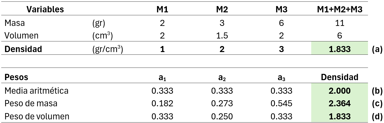
This indicates that the unit in which the variable value is measured lies in the denominator; therefore, to average the variable, we must consider the denominator to obtain the value of the variable in the mixture.

With this, we are ready to generalise the additivity of variables: a variable will be additive if the sum of its parts allows us to obtain the total value, such that y=a₁x₁ + a₂x₂ +…+ a_nx_n, where the following restrictions apply: if we have an extensive variable, then a₁ = a₂ = a_n=1, and if it is an intensive variable, then a₁ + a₂ +...+ a_n   =1.

Other Properties

We already mentioned that linearity allows us to calculate the total mixture from individual samples and to determine whether a variable is additive or not by comparing calculated and measured mixtures. Linear functions exhibit the superposition principle, meaning that the total response of a sample equals the sum of individual responses from its subsamples (note that we are calculating mixtures, not performing estimations).

This linearity also applies to variables derived from functions of other variables: for such a derived variable to be additive, the underlying function must be linear (so far, we have assumed the original variables are additive). If a variable cannot be obtained through a direct sum or weighted average, it is non-additive. Examples of non-additive variables include those defined by logarithmic or exponential dependencies.

Non-additive variables are those whose mean value cannot be obtained through a direct sum or weighted average due to their non-linear behaviour. Examples include resistance and permeability, where the mean does not faithfully represent the physical reality.

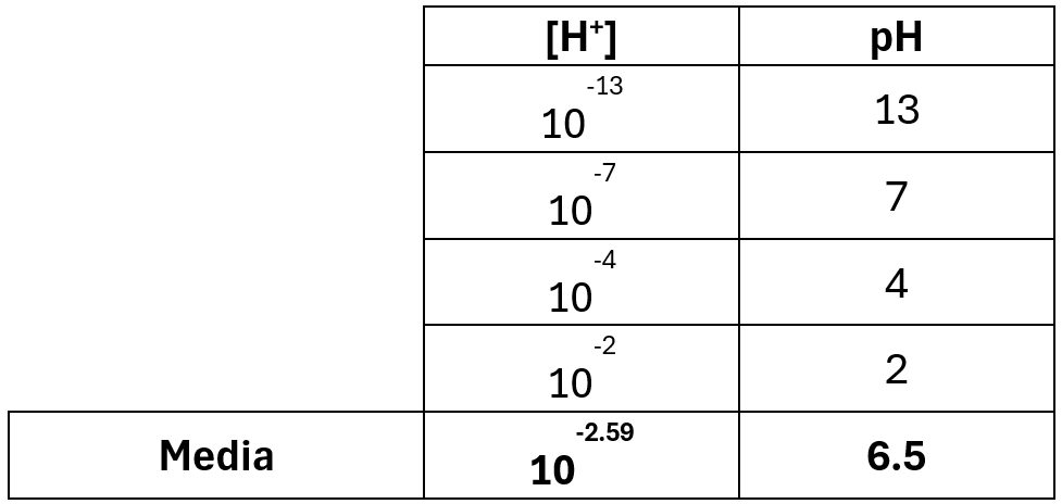
Let’s examine this with the variable pH. In Table 2, pH is defined as pH = -log₁₀[H⁺]. If we take the arithmetic mean directly from pH values, we get 6.5; however, if we compute it from the concentration, the resulting pH is 2.59. This shows that averages cannot be derived from non-linear functions — the definition must be used to obtain correct results. In this case, the weighted average is derived from the hydrogen ion concentration, which is then transformed into pH.

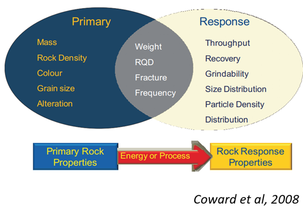
There are other properties of variables in areas such as geotechnics or metallurgy that can be classified as primary or response properties. A primary property represents an intrinsic characteristic of the studied material, while a response property represents a characteristic of the material’s response to a process. Between both classifications, there are intermediate properties (see Figure 1).

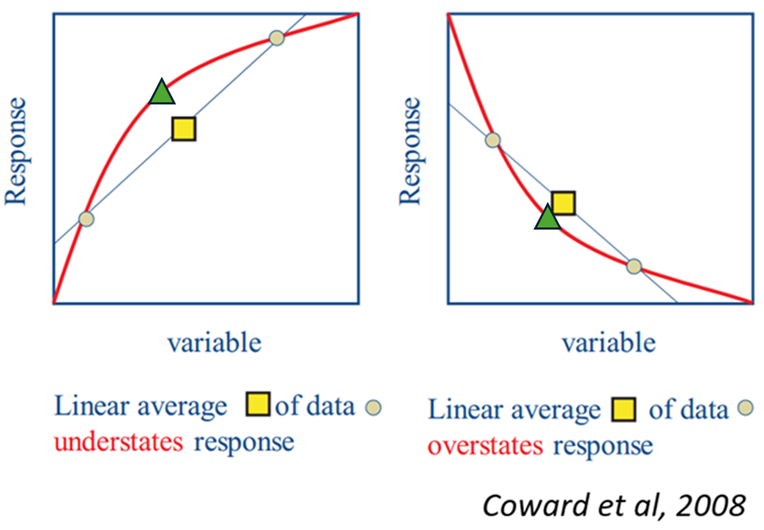
Response variables correspond to measured results in a test and can be influenced by factors not included in their definitions. In general, response variables are complex and non-linear.

In Figure 2, the effect of calculating a response variable (square) from two samples (circles) is shown: because the behaviour is non-linear, the mixed value does not match the actual response (triangle). Later, we will revisit this issue using the Work Index variable.

Linearity in Estimation Function

An area related to the additivity of variables is geostatistics, which is the branch of statistics that analyses and models the spatial variability of phenomena and focuses on the spatial dependence of data — that is, how the location of one measurement affects others nearby. Unlike classical statistics, which considers data independent of space, geostatistics studies regionalised phenomena (that is, the behaviour of variables within a given volume).

Most methods used in geostatistics involve calculating spatially weighted arithmetic means. Unlike the additivity discussed earlier, which relates to sample mixtures and the value derived from initial samples in the mathematical space defined by the variable, here the focus is on spatial dependency.

Next, we will review the kriging and simulation equations to understand their relationship with additive variables.

The general form of an estimation function is:

Z(r)=b₁*Z(r₁) + b₂* Z(r₂) +...+ b_n* Z(r_n) 

In estimation, the weights (b₁…bₙ) are related both to the variable values and their spatial relationships, which are defined by their variogram behaviour.

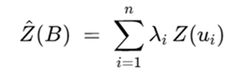
For the case of ordinary kriging, the equation is defined as:

And for conditional simulation, as:

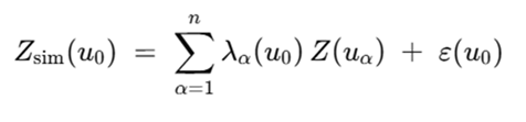
Both functions are linear, which means that the input variables must be additive — and therefore linear. This is why understanding the additivity and linearity of variables is essential. The linearity required in estimation is defined in a three-dimensional space. For the example of density, additivity is defined in space (volume), and because its estimation also requires spatial linearity, it fully satisfies the conditions for estimation.

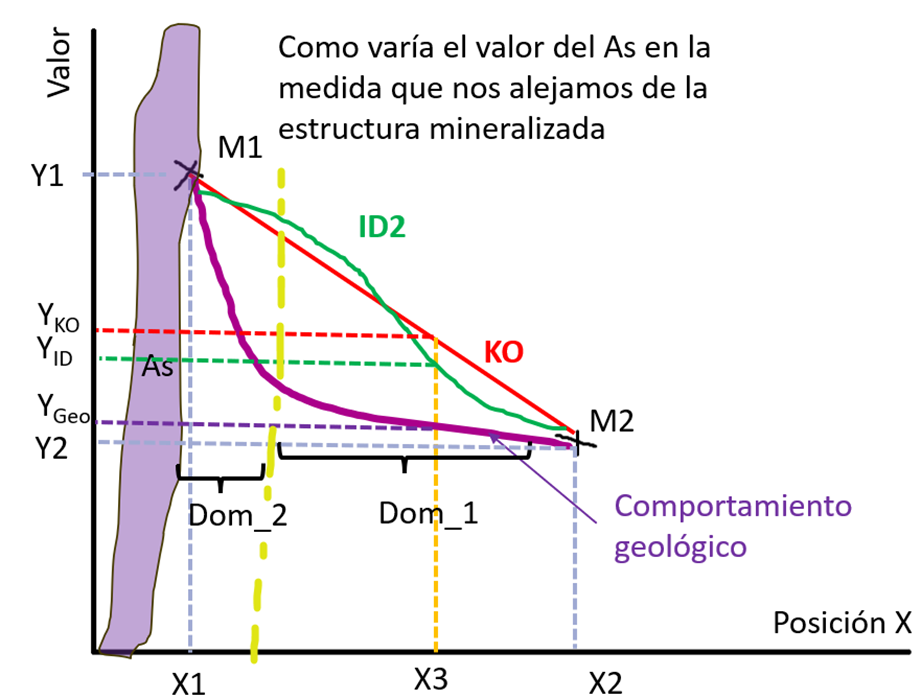
Now let us examine the spatial behaviour of a variable across different domains. In the following example, we look at how arsenic (As) behaves as we move away from an enargite (Cu₃AsS₄) mineralised vein. We have two samples (M1 and M2) with As concentrations and want to determine the grade (Y) at X3 (Figure 3). The red line represents the ordinary kriging (OK) estimation — a linear function; the green line represents inverse distance squared (ID²) estimation — a non-linear function; and the purple line shows the real arsenic behaviour.

From this example, we can infer that, when using linear interpolation models on non-linear variables, it is necessary to define at least two domains between X1 and X2 so that the variable behaves approximately linearly within each domain. This is because the variable’s behaviour is non-linear under certain conditions (e.g., contact between a mineralised dyke and host rock). This example illustrates the linearity of the OK function, the non-linearity of the ID² function, and the non-linear behaviour of the variable itself — but by constraining the domains, we can assume approximate linearity to apply estimation methods.

In the next blog, we will present examples of geotechnical and metallurgical variables to better understand these types of non-additive variables — their definitions, behaviours, and how to approach their estimation under the inherent constraints of each variable.