Additive and Non-Additive Variables III: Reviewing Additivity and Linearity Properties of Percentage-Type Concentrations
This is the final entry related to additive and non-additive variables. Remember that you can find information on non-additive geotechnical and metallurgical variables in our previous post.
Are Cu (%) concentrations additive and linear?
Below, we will review percentage-type concentration variables defined by:
Concentration (X) % = 100 *(masa)X/(masa)Tot, that is, the amount in grams of the element of interest (X) relative to the total mass of the sample ((mass)Tot), multiplied by 100 to obtain the concentration in %. Table 1 presents two samples used to determine their additivity. They are separated into three components to later understand the effect of density. Sample M_01 weighs 100 grams (see row b), with 1 gram of Cu (see row a), 15 grams of Mag, and 84 grams of gangue, resulting in 1% Cu (see row c). For sample M_02 the result is 2% Cu. In the last column, both samples are mixed, and applying the definition, a grade of 1.67% Cu is obtained.
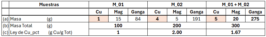
To demonstrate its additivity, we must obtain the same grade for the mixture of samples M_01 and M_02 using the definition y=a1x1 + a2x2 +…+ anxn. The weights a1…an are given by the denominator of the concentration definition, which is the total mass. Thus, the Cu concentration of M_01 + M_02 is:
Cu% M_01 + M_02 =(100gM_01/300gM_01_M_02) *1%CuM_01+(200 gM_02/300 g M_01_M_02) *2%Cu M_02=1.67
The obtained value is the same as that derived by applying the percentage-grade definition and presented in Table 1 using the sum of samples M_01 and M_02. Therefore, we are dealing with an additive variable; specifically, it is additive in the space of the total mass defined in the concentration (X) % formula.
Now, when we use this variable to perform spatial estimations, these are carried out in 3D Euclidean (volumetric) space, and it is in this space—Euclidean or volumetric—where a linear behaviour of the data is assumed for OK equations or simulations.
As a first step, we will review the concentration of X (Cu, for example) in total-mass space and in volumetric space to understand how these values relate or behave.
To simplify the grade expressed between 0 and 100%, we will express it between 0 and 1.
Concentration of (X) in total-mass space:
(X) = (masa)Cu/(masa)Tot
Concentration of (X) in Euclidean space:
(X) = (masa)Cu/ (volumen)Tot = (masa)Cu/ (masa/ρ)Tot ,
where (masa)Cu = metal of interest, (masa)Tot = total sample mass, (volumen)Tot = total volume, and (masa/ρ)Tot = total sample mass divided by the sample density.
Using these relationships, we can transform concentrations defined in total-mass space into concentrations in Euclidean space.
For this exercise, only the denominator of the definition (the total sample mass, (masa)Tot) is replaced using the density definition, because the densities of different samples vary and will depend on the composition of the minerals present. Meanwhile, the numerator is not replaced using the density definition because the density is the same in all samples for the analysed metal, as it is the same element and therefore has a constant density.
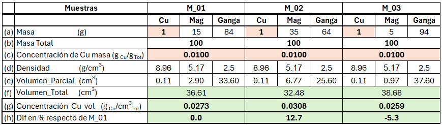
To begin, we will transform the Cu grade of three samples (M_01, M_02, and M_03) for visualization. Table 2 shows that each sample contains Cu, magnetite, and gangue, together with their respective densities (d) and masses (a). Concentrations are expressed as mass ratios (c) within total-mass space. Using the densities of each component (e), we convert masses into volumes to obtain the total volume (f), thus applying the volumetric concentration definition in Euclidean space.
If we compare the volumetric concentration of samples M_02 and M_03 with that of sample M_01, the first observation is that volumes differ among them, as do their volumetric concentrations (h). Thus, while in total-mass space the concentrations are equal for all samples, in volumetric space the same samples display different concentrations due to the effect of varying densities.
From this exercise, we see that when estimating concentrations, the assumption of linear behaviour impacts differently depending on the space in which the estimation variable is defined. When linearity is applied to the variable defined in total-mass space, we implicitly require that both the amount of Cu and the sample density vary linearly together—something difficult to justify conceptually. In contrast, when linearity is assumed for the concentration variable defined in volumetric space, what is required is that the Cu content behaves linearly in space; this is reasonable, since both the estimation space and the variable are defined in volumetric (Euclidean) space.
In the case of the variable defined in total-mass space, the Cu content is only known once density is estimated, which implies that the final amount of Cu directly depends on that estimation. This is relevant, because density estimation does not always receive enough attention, despite its impact on results.
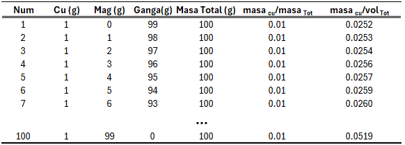
To visualize the relationship between the concentration variables defined in total-mass space and volumetric space, Table 3 was constructed using the previous definitions. This table contains 100 samples with a constant total mass of 100 g. Each sample is composed of Cu, magnetite (Mag), and gangue. The Cu content is constant in all samples (1 g), while the amount of magnetite increases progressively from 0 g to 99 g, with the gangue reduced proportionally.
For each sample, the Cu concentration is calculated both in total-mass space (mass Cu / total mass) and volumetric space (mass Cu / total volume).
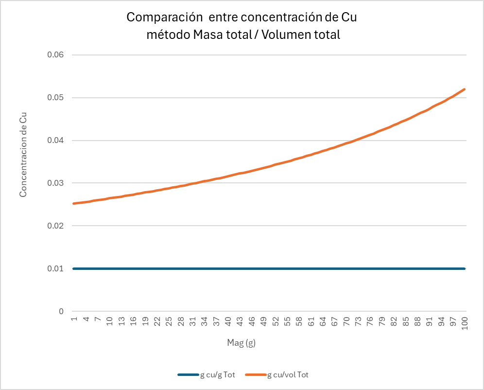
From this table, the graph in Figure 1 is generated. It shows that the definitions of both variables do not exhibit linear behaviour. While the variable defined in total-mass space remains constant, the concentration defined in volumetric space increases as density increases (due to the higher magnetite content). Additionally, the graph shows that the relationship between the two variables is also non-linear.
In the next graph (Figure 2), generated from a table similar to the previous one but composed only of Cu and gangue, the Cu content is progressively increased and two variables are represented: Cu concentration defined in volumetric space and Cu concentration defined in total-mass space. The result shows that the relationship between these two variables is non-linear.
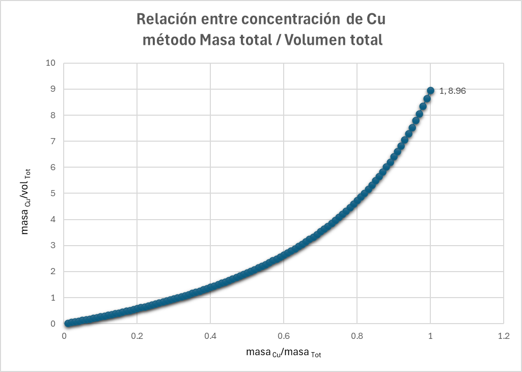
In summary, both variables are additive in their respective spaces (total-mass space and volumetric space). For both, we must assume linearity when estimating (whether by kriging or simulations). However, for the concentration defined in total-mass space, the Cu concentration relates non-linearly to the Euclidean (volumetric) estimation space due to variations in density between samples. The relationship between both types of concentration is expressed as: CuV concentration = CuM concentration × (massTot / volTot).
This raises the question: how can we control this non-linear behaviour of the data in Euclidean space? If density were constant across samples, the non-linearity would disappear. For this reason, one strategy is to define appropriate domains that reduce density variability. Similarly, samples with very different densities can be treated as outliers. Furthermore, as a corollary, the critical importance of correctly estimating density is reinforced—density determines the amount of Cu present in the deposit.
Finally, although volumetric concentration is fully compatible with the estimation space and allows the Cu content to be obtained directly without involving density, it presents a practical disadvantage: measuring total volume is extremely difficult. For this reason, the variable that is actually measured and used is the one defined in total-mass space. Even so, performing comparative exercises between both concentration definitions is highly recommended, as they help us better understand the variables we use routinely and, above all, recognize their limitations so that definitions, procedures, calculations, and estimations are applied correctly.
With this, we conclude the series on additive and non-additive variables. We hope it has been of interest and that it has allowed you to delve deeper into these concepts. We invite you to stay tuned for our upcoming publications.