Case Study: Validating Machine Learning Models in Mining

Validating Predictive Models in Mining

This article addresses the validation of predictive models in mining. In a previous article, we reviewed hyperparameter optimization as a way to obtain models that perform well on unseen data. However, optimization is only one part of the process: it allows us to select a candidate model, which must then be validated to determine whether it is suitable for operational use. To show how this validation is carried out with operational relevance, we will follow a specific case: a model that predicts plant recovery.

Reconstructing the Processed Material

In this type of project, validation begins by reconstructing the processed material. To do so, we work with four main data sources:

Ore movement records: indicate the origin and tonnage of the material fed during each period.
Extraction polygons: identify the areas, phases, and benches from which the ore originates.
Block model: provides the geological and geometallurgical characteristics of the extracted material.
Stockpile information: describes the stored material that is subsequently incorporated into the plant feed.

By integrating these four sources, we can reconstruct the processed material, apply the model, and compare its predicted recovery with the recovery recorded by the plant. From this reconstruction, validation proceeds at two levels: first, the model's predictive capability is evaluated on held-out data; then, we assess whether it adequately represents the blend that reaches the plant.

Note: to protect confidentiality, the figures in this article use artificial data built from operational patterns that were rescaled, shifted, and perturbed; they preserve no dates, values, or results from any specific operation.

First Level: Predictive Capability on Held-Out Data

The first level evaluates the model on a test set that was used for neither training nor optimization. Each point represents an observation reserved for this evaluation. Rather than relying on a single metric, we use a panel with several complementary views.

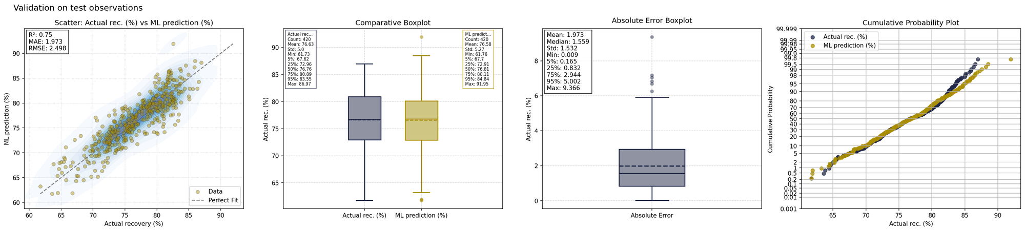
Figure 1: Diagnostics on the test set: actual-versus-predicted scatter plot with density, comparative boxplots, absolute error, and cumulative probability. The R² in this example is 0.75.

Each component provides different information:

Actual-versus-predicted scatter plot with density: each observation is positioned according to its actual and predicted recovery relative to the 1:1 identity line. Density shows where most of the data are concentrated, and R², RMSE, and MAE are also reported in the panel to summarize goodness of fit and error magnitude.
Comparative box plot: compares the distributions of actual and predicted recovery. Similar medians, spreads, and ranges indicate that the model reproduces the overall distribution of the target, rather than only individual observations.
Absolute error box plot: summarizes the magnitude of the differences between actual and predicted values. A low median and a limited number of extreme errors are desirable.
Cumulative probability plot: compares both distributions across their full range, helping reveal differences that may not appear in global metrics.

This panel covers the first level of validation: predictive capability on held-out data. However, completing the case evaluation requires checking whether that performance is maintained when representing the material that actually reaches the plant.

Second Level: The Shift in Scale Toward the Plant

This is where the main change in scale arises. The model predicts at the scale of a sample, a block, or another characterized unit, while the plant processes a blend from different phases, benches, and stockpiles. A model may predict those units well individually and still fail to reproduce plant recovery if the actual blend is not reconstructed correctly.

Reconciliation addresses precisely this change in scale: the same model evaluated on the test data is now applied to the characterized material from the block model and stockpiles, and its predictions are then matched with movement records and feed tonnage. Recovery for each period is calculated by weighting contributions by tonnage and head grade, that is, by their metal content, which represents the metallurgical balance more faithfully than a simple average.

Information coverage is also part of the calculation: for each period, we determine what proportion of the feed tonnage could be characterized using mine or stockpile information. Only periods that exceed a minimum coverage threshold are interpreted, because a reconciliation based on a small fraction of the feed can produce misleading results.

Once the processed blend has been reconstructed, the time scale for comparison is defined. Although plant recovery is recorded daily, those values also reflect shutdowns, residence times, feed changes, and measurement variability that the geometallurgical model is not intended to explain directly. For this reason, reconciliation is performed at a weekly scale: aggregation reduces some of the daily noise and makes the signal associated with the processed material easier to observe.

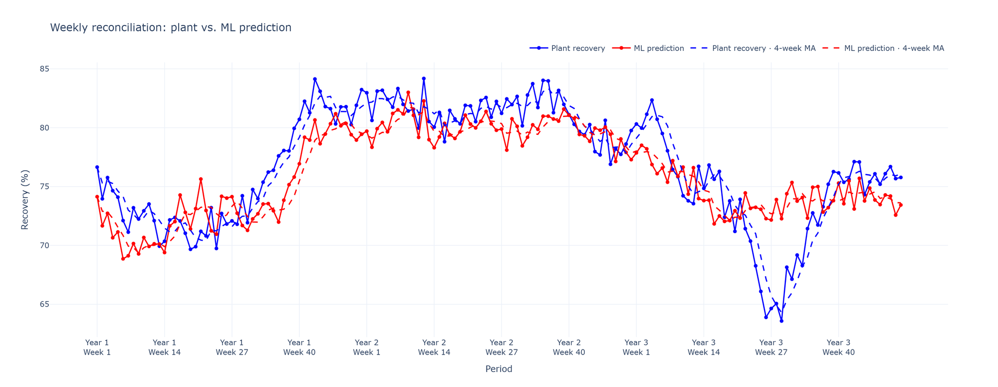
Figure 2. Plant recovery and model prediction at a weekly scale, together with their four-week moving averages.

Interpreting the reconciliation involves more than assessing the proximity of the curves: we also examine level changes, sustained bias, coverage, and the magnitude of the differences. An isolated divergence may be associated with an operating condition not represented by the ore characteristics, but this hypothesis must be checked against process records before assigning a cause.

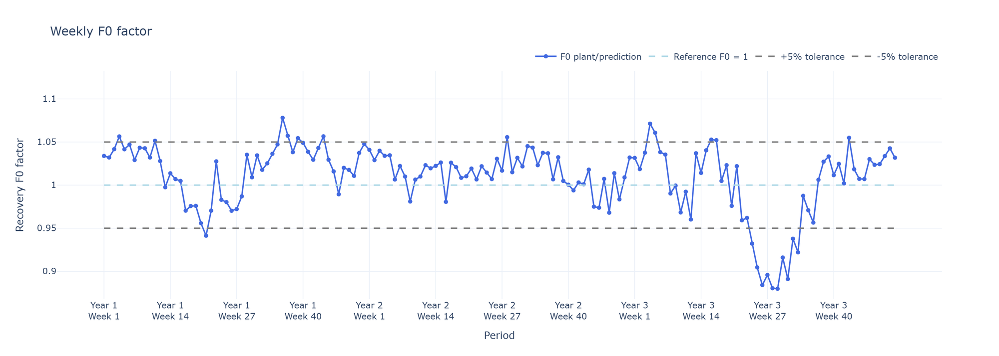
To complement this time-series view, the same comparison can be expressed as a ratio using the F0 factor, calculated as plant recovery divided by predicted recovery. A value of 1 represents agreement; values above or below 1 indicate the relative deviation from the prediction. Unlike the time series, F0 directly identifies periods that fall outside the tolerance defined for reconciliation.

Figure 3. Weekly F0 factor. The ±5% bands are reference tolerances, not statistically estimated control limits.

Three Views, One Process

The three views presented are connected within a single process: the test panel measures statistical performance, reconciliation assesses how the model behaves when representing the processed blend, and the F0 factor summarizes the relative deviation between actual and predicted recovery. Together, they follow the model from predictive evaluation through to its application in the plant.

This workflow addresses the specific objective of predicting recovery and is not a universal methodology. Each type of project requires its own validation process, adapted to the predicted variable, the scale at which the model will be used, and the operating conditions. For plant recovery, reconciliation by tonnage and metal content is appropriate; estimating rougher recovery, mineralogy, or comminution variables, on the other hand, requires different scales, metrics, and acceptance criteria.

A Multidisciplinary Effort

Designing such an adapted process requires different disciplines to work together: the data scientist designs the evaluation and quantifies the error, while geologists provide the knowledge needed to represent the material and judge whether the comparisons make geological sense. Model validation arises, precisely, from the integration of these disciplines.

This joint perspective makes it possible to distinguish between selecting a good model and demonstrating that it can be used in operations. Hyperparameter optimization allows us to select a candidate model; validation determines whether that model can be used in a specific operational context. The plant recovery case illustrates the central idea: a model is not considered reliable simply because it achieves a good metric on test data, but because it passes a validation process designed specifically for the problem and the particular conditions of each project.