educational blog

Beyond Kriging: the Role of Conditional Simulations in Resource Evaluation

In recent years, conditional simulations have been gaining increasing importance in Mineral Resource evaluation and are being more frequently required in projects and operating mines, due to their multiple uses. However, their greater complexity means that they are not yet used across the board in the industry. In the following blog we will learn what they are, how they differ from traditional linear estimators and some of their uses in real cases worked on by GeoEstima.

What are geostatistical simulations?

They are an application of the Monte Carlo simulation to regionalized variables that allow quantifying the model’s uncertainty. Geostatistical simulation techniques generate a group of realizations or realities with equal probability of occurrence. If there is greater variability in the data or there is less data to generate a model, the realizations will have a greater degree of difference between them (Abzalov, 2016).

Depending on their application they can be used for categorical variables (lithology, mineral zones, alterations) or for continuous variables (grades, density, recoveries) (Rossi & Deutsch, 2014; Chiles & Delfiner, 2012). Normally, we will use conditional simulations which restore the measured values in the sites with data, therefore these sites with information will not have uncertainty (Emery, 2015).

The generated models have the particularity of reproducing the data distribution or histogram (proportion of high, low values, median and variance) and the variogram (spatial continuity, anisotropies and nugget effect) (Rossi & Deutsch, 2014). The idea of conditional simulations is to build a representation of the phenomenon that is consistent with the data and that reproduces the local fluctuations: it is not reality, but it is a possible version of it (Chiles & Delfiner, 2012).

Some practical considerations that must be taken into account include the necessity of calculating the declustering weights of the samples to obtain the representative distribution of the phenomenon and not a biased distribution due to preferential sampling. Another important factor is the definition of domains, given that conditional simulations are sensitive to non-stationarity. To use simulations, it is necessary to previously transform the data to Gaussian space (mean zero, variance one), which is done through a function called anamorphosis. Finally, the simulations represent the grades or values at point support, and their results must be re-blocked and averaged to the support of interest (SMU).

There are different geostatistical simulation algorithms available in many of the commercial software. Some simulations techniques for continuous variables are the sequential Gaussian algorithm (SGS) or the turning bands algorithm (TB). Similarly, some of the popular algorithms for simulating categorical variables are the sequential indicator simulation (SIS), multipoint simulation (MPS) or the hierarchical truncated pluri-Gaussian simulation (HTPG)

Estimation vs simulation

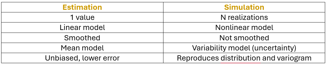
The estimations give a value that on average approaches the unknown reality. It is a linear combination of the available data, unbiased, with the lowest mean squared error and inevitably exhibits smoothing (greater minimums and lowest maximums than the data). The estimations will give the expected value.

The simulations, on the other hand, are non-linear models, they reproduce the data variability, which means that extreme values are preserved (no smoothing). The simulations give a set of values for each point, which allows quantifying the uncertainty. The simulations will reproduce correctly the proportion of high and low values.

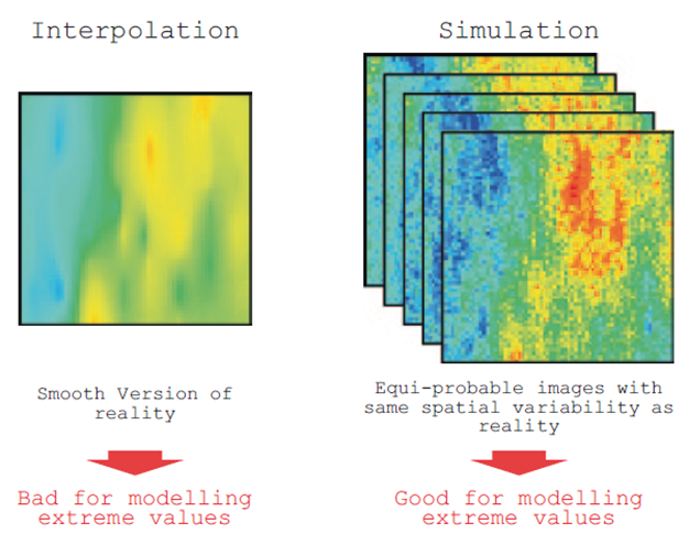
Table 1: Comparison of Estimations and Simulations

In the Figure 1 it can be seen how the estimated model, being smoothed, shows higher minimum values and lower maximum values, meanwhile simulations, not being smoothed, reproduce better the low and high values. Additionally, it is observed how the estimation is just one model, while simulations are N models with the same occurrence probability.

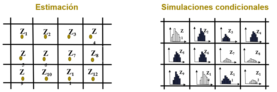
Figure 1: Estimation vs simulation (Rossi & Deutsch, 2014)

As mentioned, the estimations provide one unique value for each block of the model, while the simulations, being N models, give a value distribution for each block (Figure 2).

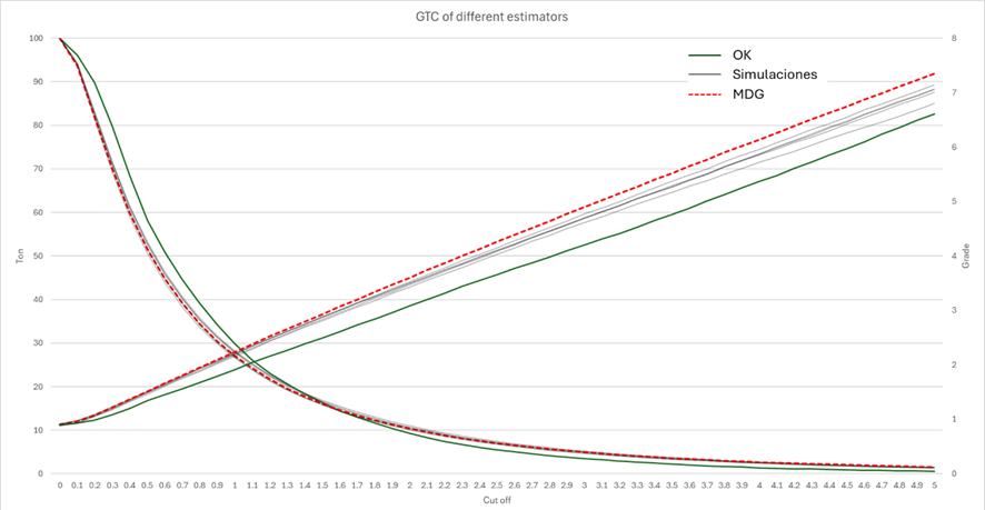
Figure 2: Estimation vs simulation for each block

If the discrete gaussian model is used as a reference, the difference between a kriging estimated model and a simulated model in terms of the tonnage/grade curve can be observed: the kriging, due to smoothing, reports more low-grade tonnage and less high-grade tonnage, while the simulations do not have these deviations. In the same way, the kriging always reports a lower mean grade at cut-off grades greater than zero (it is only unbiased at cut-off 0), unlike conditional simulations. For this comparison the point simulations were averaged to the SMU support, the same one as that of kriging.

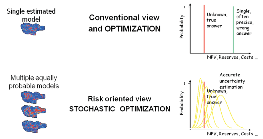
Figure 3: Tonnage-Grade curve: traditional model vs simulations

Why use simulations?

Due to the high risk that constitutes any mining project, the uncertainty and the resulting risk must be quantified for better decision-making.

The advantage that simulations have over traditional estimations is that they allow the generation of uncertainty models from which different types of studies can be conducted: risk analysis, uncertainty quantification of both geology and grades, resource category definition, mineralization potential studies, drill hole spacing optimization studies, and more recently, stochastic planning.

How to properly integrate them into the workflow?

Although simulations are usually used to quantify grade uncertainty, limiting the simulation study to nothing more than that is a mistake, since the goal should always be to integrate the highest number of uncertainty sources in the model to avoid having only a partial view.

When possible, it is recommended to quantify variability at each stage of the resource study, following the hierarchic workflow and one to one realization configuration. Figure 4 schematically shows the integration of uncertainty at the different stages of the model, following the one-to-one configuration, transferring the uncertainty at each stage (Deutsch, 2018; Deutsch, 2021).

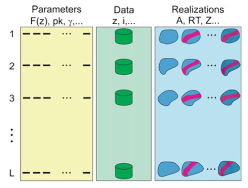
Figure 4: Simulations at each stage of the workflow (Deutsch, 2021)

Data uncertainty: for multivariable studies, if heterotrophic databases are available, it is recommended to impute the missing data by generating realizations of these and integrating these realizations one-to-one into the study.
Parameter uncertainty: it is possible to perform spatial Bootstrap to quantify uncertainty in the data histogram.
Geological uncertainty: geology has intrinsic variability that will directly impact the mineralized volumes and the reported tonnage, which is why quantifying contact variability is crucial to understanding the total variability of the phenomenon being modeled.
Grade uncertainty: this is the workflow stage that is usually performed; it involves the uncertainty quantification of the grades of interest (economic minerals and pollutants when applicable). If it is a multivariable study, a decision must be made between performing co-simulations or simulating independent factors (transformations such as PPMT, projection pursuit multivariate transformation, or MAF, Min-max autocorrelated factor), so that the resulting simulations maintain the data correlations and other complex structures in the data due to heteroscedasticity or no-linearity.

Thus, by integrating uncertainty at each successive stage, the result will be a much more faithful reflection of the total variability of the process, and the subsequent analysis performed will be much more robust.

Application examples

The following are practical cases from large-scale mining operations in which simulations have delivered good results and led to better decision-making.

Geological uncertainty quantification

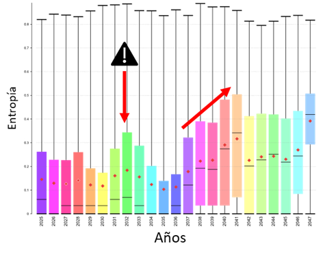
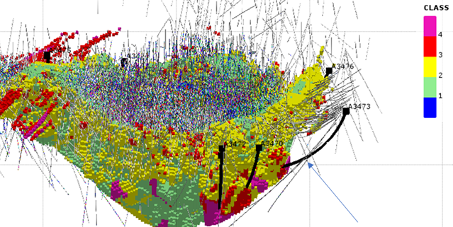
From the conditional simulations, the entropy variable has been calculated, which summarizes the geological model uncertainty. From this, it is possible to define the zones where the model is more uncertain and therefore requires a greater amount of information (drillholes) to be correctly characterized (Figure 5). This can help with planning new drilling campaigns (Figure 6) or taking mitigation actions, such as blending material from different zones or adjusting the plan to avoid sending different fronts with high entropy to the plant.

Figure 5: High entropy zones in the mining plan

Figure 6: Recommendation of new drill holes (in black) in zones of high geological uncertainty

Grid studies for resource categorization definition

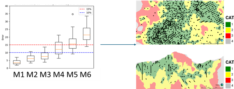
From a simulation study, artificial sampling and re-simulation, it is possible to quantify the relationship between drillholes spacing and uncertainty, in other words, this allows measurement of how much the deposit variability will decrease with the arrival of new information. If this is related to a tolerated error and a confidence level, the drillhole grids necessary for the measured and indicated categories can be defined. The advantage of this study compared to other categorization tools is that the uncertainty is directly measured and the variability of both geology and grades is integrated. Additionally, it allows measurement of the error above a cut-off grade.

Figure 7: Uncertainty vs spacing and resource categorization

Short-term risk analysis

From the simulated model, an indicator was generated with 90% confidence of being mineralized rock and exceeding the operational cut-off grade. This indicator was crossed with the official resource model, and blocks were identified where the deterministic model showed mineralized rock exceeding the cut-off grade, but the simulations indicated a low probability of this being the case. When checking this indicator against the reconciliations, a correlation was observed between the indicator and poor performance of the official resource model. In this way, the indicator was used by the short-term planning team to identify phases and benches close to mining with a high probability of error (red blocks in Figure 8).

Figure 8: Indicator in red: high-risk zones (low probability of being as planned)

Stochastic planning

The simulated models of geology and grades can be used as input for stochastic planning algorithms. Recently, GeoEstima completed a model for a world-class Cu deposit in which the mineral zones, lithologies and Cu, CuS and Mo grades were simulated. Together, these 100 models will be used to integrate deposit uncertainty into the mine design, production plan and economic evaluation of mining and operational projects. Stochastic workflows increase total tonnage by up to 15% compared to the traditional planning. Additionally, an increase of up to 10% in VAN between stochastic and traditional planning has been demonstrated (Dimitrakopoulos, 2018).

Figure 9: Traditional vs stochastic approach (modified from Dimitrakopoulos, 2018)

Conditional simulations are revolutionising the way we understand uncertainty in mining. Have you worked with them? Would you like to know how they can help you make better decisions and reduce risks in your projects?

References

Abzalov, M. (2016). Applied mining geology (Vol. 12).
Chiles, J.-P., & Delfiner, P. (2012). Geostatistics : Modeling Spatial Uncertainty. John Wiley & Sons.
Deutsch, C. V. (2018). All Realizations All the Time. In Handbook of Mathematical Geosciences (pp. 131–142). Springer International Publishing. https://doi.org/10.1007/978-3-319-78999-6_7
Deutsch, C. V. (2021). Implementation of Geostatistical Algorithms. Mathematical Geosciences, 53(2), 227–237. https://doi.org/10.1007/s11004-020-09884-z
Dimitrakopoulos, R. (2018). Stochastic Mine Planning—Methods, Examples and Value in an Uncertain World. In: Dimitrakopoulos, R. (eds) Advances in Applied Strategic Mine Planning
Emery, X. (2015). Geoestadística. Ingenierìa de Minas, Universidad de Chile.
Rossi, M. E., & Deutsch, C. V. (2014). Mineral Resource Estimation. In Mineral Resource Estimation. Springer Netherlands. https://doi.org/10.1007/978-1-4020-5717-5