Integration of Different Data Supports in Short-Term Estimation
The problem: data of different quality and support
In mining projects, it is common to simultaneously have two or more sources of geochemical information that differ in both sampling density and physical support: exploration drillholes (DDH or RC), collected throughout the life of the project with relatively wide spacing, and blast holes (BH), sampled extensively during the production stage with increasingly dense patterns as mining progresses. Both sources contain valuable information; however, integrating them without proper care may introduce significant bias into the resource model.
The central question is: how can the high spatial density of blast holes be leveraged to improve grade estimation based on drillholes without compromising the unbiasedness of the estimator? The answer lies in co-kriging; however, its proper application requires first understanding several fundamental statistical and geostatistical concepts.
Volume–variance relationship: bias and quality
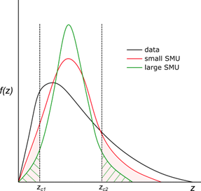
The physical support of a sample—its volume—directly affects its statistical variability. A blast hole represents a rock volume on the order of tens of tonnes, whereas a 2 m composite DDH sample represents only a few kilograms. Due to the volume–variance relationship, samples with larger support exhibit lower variance and more symmetrical distributions than those with smaller support (Donovan, 2015; Minnitt & Deutsch, 2014).
This implies that directly comparing the statistical distributions of DDH and BH samples may lead to incorrect conclusions regarding bias between the two sources. Secondary samples of exhaustive type—such as blast holes—are subject to their own sources of bias, imprecision, and error. Donovan (2015) identifies three main stages where these issues may arise: sample collection, laboratory analysis, and data preparation by the analyst.
Comparing distributions from fully heterotopic sources
Before formulating any co-kriging model, it is essential to assess the statistical comparability between the two data sources. This is achieved using multivariate graphical tools and formal statistical tests, which together help identify systematic bias and distributional differences.
The key question is whether two samples originate from the same distribution, or equivalently, whether there is a systematic difference in the measured magnitude. Distributions may be characterized by their shape, location, and scale.
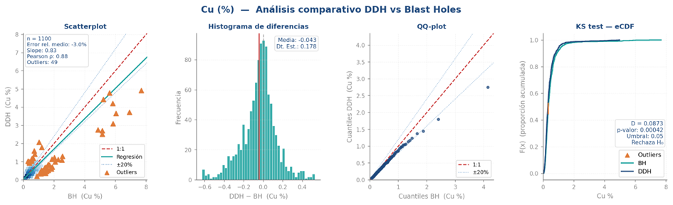
Scatter plots allow visualization of linear correlation and identification of outliers or systematic groupings, while overlaid QQ-plots reveal quantile-to-quantile differences between distributions.
To complement graphical analysis, hypothesis testing is applied. The Kolmogorov–Smirnov (KS) test evaluates whether two samples come from the same distribution by measuring the maximum difference between their cumulative distribution functions. It is non-parametric and robust to non-normality, though less sensitive in the tails. The Anderson–Darling test is more sensitive to tail differences, making it preferable when high grades have greater economic impact.
In practice, no single test is conclusive. The recommended approach is to combine all tests with visual analysis. When samples are not co-located, “twin” pairs are constructed using a spatial buffer, pairing samples from both supports within a defined proximity window.
Additionally, the correlation coefficient between paired samples is a critical practical criterion for defining the integration strategy. Following Minnitt and Deutsch (2014) and Donovan (2015): correlation > 0.8 → datasets can be directly combined; 0.7–0.8 → standardized ordinary co-kriging (SCOK) typically improves estimates; and < 0.7 → efficiency becomes questionable.
Homotopy and heterotopy
In multivariate geostatistics, two variables are said to be homotopic when each sample of one variable has a co-located sample (same location) of the other. In practice, this rarely occurs for information of different supports: DDH and BH sample different locations of the deposit. This condition is called heterotopy and has direct consequences on how spatial modelling and estimation of both variables will be carried out.
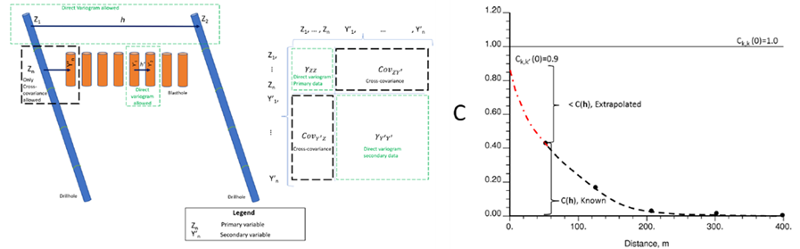
When data are fully heterotopic, the experimental cross-variogram between drillholes and blast holes cannot be calculated, as no co-located pairs exist; the experimental cross-variogram can only be calculated from homotopic data. The equation of the cross-variogram defines that the information of the primary variable “Z” and secondary variable “Y” must be obtained at the same location “u”:

To deal with this, there are some alternatives:
- Extrapolation of covariance and inference of the cross-variogram: according to Davila & Deutsch (2022), cross-covariance can be calculated and extrapolated to the origin in distance:

and the cross-variogram can be inferred (Cuba & Deutsch, 2012). This detail has practical importance: a poorly extrapolated cross-correlation overestimates or underestimates the contribution of the secondary variable to the estimator.
- Direct Linear Model of Coregionalization (LMC) of cross-covariances for n distances.
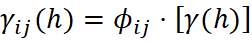
- Intrinsic Coregionalization Model (ICM), a particular case of LMC where the regionalized correlation coefficient is the same for both scales (correlation is independent of spatial scale). In this case, direct and cross-variograms are proportional to the same variogram:

with one or more structures:
The Linear Model of Coregionalization (LMC)
For any co-kriging variant, direct variograms and the cross-variogram must be modelled jointly in a consistent way. This requirement is formalized in the LMC, which decomposes each variogram into N nested structures. The indispensable condition is that the coefficient matrix:

is positive semi-definite for each structure N. In the bivariate case, this reduces to requiring that the condition holds:
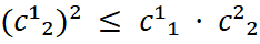
per structure. If this condition is violated, the co-kriging system may produce negative variances.
In practice, the simultaneous fitting of the LMC with three variograms (direct and cross) is the most laborious part of the workflow. Tools such as Isatis.neo, RMSP and other geostatistical software allow interactive fitting with automatic validation of the positive semi-definite condition. An alternative for multiple correlated variables is decorrelation through PCA/MAF/PPMT factors, allowing independent modelling and simulation of each factor.
The Intrinsic Coregionalization Model (ICM)
The Intrinsic Coregionalization Model (ICM) is a particular case of the Linear Model of Coregionalization (LMC), in which all direct and cross-variograms of the variables under analysis are proportional to a single base variogram. This variogram may be composed of one or more fundamental structures, following the mathematical property below:
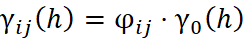
where:

represents a variogram model with unit sill;

is the direct or cross-variogram between variables i and j;

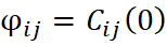
is the proportionality coefficient between the variograms of the different variables;

is the value of the covariance matrix at zero lag.
In this context, the ICM simplifies the modelling of spatial dependence among multiple variables by assuming that all variables share the same underlying spatial structure, differing only by proportionality coefficients. This approach reduces the computational complexity of multivariate geostatistical modelling while ensuring statistical consistency between direct and cross-variograms.
Multivariable estimation methods: co-kriging
Co-kriging is a generalization of kriging for multiple variables that provides a minimum-variance unbiased estimator. This method incorporates spatial correlation between variables through the cross-covariance function, allowing the use of secondary information without the need for exhaustive sampling. Data may be located at the same points as the primary variable or distributed at different spatial locations, making co-kriging a flexible approach for multivariate geostatistical modelling.
The objective is to improve the estimation of the primary variable by incorporating information from more densely sampled secondary variables, particularly when the primary variable exhibits low spatial autocorrelation while the secondary variables display greater spatial continuity.
A key benefit of co-kriging is the reduction of estimation error variance, as it leverages the correlation between variables to improve accuracy. Therefore, the co-kriging error variance will always be less than or equal to that of simple kriging, making it more efficient for multivariate geostatistical modelling.
The simple co-kriging estimator can be defined as:
where:

and

are values of the primary and secondary random variables;

represent the means of the variables;

and

are the co-kriging weights calculated from the covariances between the primary and secondary samples.
Simple co-kriging
Simple co-kriging assumes stationary and known means for both variables. It is the most efficient in terms of variance, but it is sensitive to errors in the global means. In mining practice, it is rarely used because the means of the entire deposit are seldom known with certainty, especially in the early stages of a project.
Ordinary co-kriging
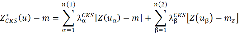
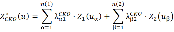
In ordinary co-kriging, the mean is assumed to be stationary only within a local neighbourhood, in contrast to simple co-kriging, which assumes stationarity over the entire study area. The ordinary co-kriging estimator for the variable of interest at a given location is expressed as:
Under the conventional conditions of ordinary co-kriging, the sum of the weights of the primary variable is equal to 1, while the sum of the weights of the secondary variable is equal to 0:
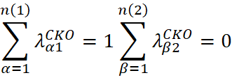
However, in practice, this restriction on the weights of the secondary variable may generate negative or very small weights, which can produce negative estimates or excessively reduce the influence of the secondary variable in the model.
Standardized ordinary co-kriging (SCOK)
Standardized Ordinary Co-kriging (SCOK), described by Goovaerts (1997), is a methodology designed to incorporate data of variable quality, considering both the autocorrelations and the spatial cross-correlations between the variables involved. This method also reduces the bias introduced by imprecise datasets by operating with standardized residuals rather than the original data, ensuring more robust and consistent estimates.
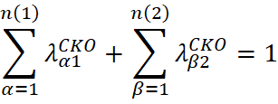
SCOK arises as an alternative to the restriction on the weights of the secondary variable in ordinary co-kriging, replacing the two previous conditions with a single constraint: the total sum of all weights must be equal to 1:
SCOK has been recommended in the mining industry for short- and medium-term estimation when integrating data of different quality (Davila & Deutsch, 2022). In fully heterotopic cases, it is common to directly model cross-covariances using the LMC, or to simplify the variogram structure through the ICM.
Collocated co-kriging
In some cases, not very frequent in mining, the secondary variable is significantly more densely sampled than the primary one, and the secondary information is already available at the location where the variable of interest is to be estimated. Collocated co-kriging is an approach that leverages this information to improve the estimation of the primary variable. In datasets where the number of primary samples is equal to or greater than that of secondary samples, the influence of distant primary samples may compromise estimation quality. This problem can be addressed using Markov Models, which propose using exclusively the collocated secondary information. Collocated co-kriging is more common when secondary information is exhaustive and is widely applied in cases where geophysical or remote sensing data are integrated into estimation.
Cross-validation: K-folds
Once the estimates are obtained, it is necessary to evaluate their quality objectively before adopting any methodology as definitive. For this purpose, cross-validation is used, which consists of estimating known locations from the remaining data and comparing the estimated value with the actual value. In the context of integrating DDH drillholes with blast holes, Donovan (2015) recommends applying this validation carefully, since the use of biased secondary data in the training set may compromise the interpretation of results if the validation set is not properly isolated. For this reason, the validation set must be composed exclusively of DDH samples, which represent the most reliable and highest-quality source, while the training set combines DDH and blast holes according to the method being evaluated.
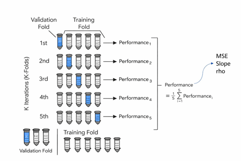
To strengthen the comparison between methods, it is recommended to apply a K-Folds cross-validation with K = 5 iterations. In each iteration, 20% of the DDH drillholes are randomly removed and used as the validation set, while the remaining 80% are combined with the blast hole samples to estimate values at the removed locations. This procedure is repeated five times so that the entirety of the DDH drillholes is used exactly once as validation, ensuring that each partition is independent and spatially representative.
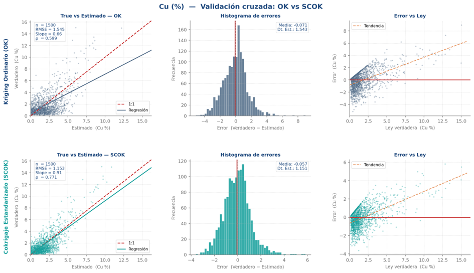
The final performance of each method corresponds to the average of the metrics calculated in each fold, considering the Pearson correlation coefficient, the mean squared error (MSE), and the slope of the regression line between estimated and actual values. The systematic comparison of these indicators across methods makes it possible to identify which technique best reproduces the primary variable with the lowest conditional bias, thereby guiding parameter selection and the final methodological decision.
Figure 4 illustrates an example of cross-validation in a comparison for Cu (%) between ordinary kriging (OK) and standardized ordinary co-kriging (SCOK).
Practical workflow and recommendations
The integration of blast holes and drillholes into a robust geostatistical model requires following a structured workflow, in which each stage conditions the decisions of the next. The critical steps of the recommended process are described below.
Comparative analysis of distributions: the starting point is the statistical comparison between the distributions of DDH and BH using pairs of samples constructed at different distances within a proximity buffer. Scatter plots, QQ-plots, and formal tests such as Kolmogorov–Smirnov and Anderson–Darling are used to quantify differences in shape, location, and scale. It is essential to identify whether there is systematic bias between the sources and to evaluate the correlation coefficient between paired samples, as this directly determines the feasibility and efficiency of any subsequent multivariate estimation.
Definition of techniques to be compared: based on the distributional and correlation analysis, it is possible to establish which strategies are applicable. When the secondary variable has greater spatial density than the primary one and the correlation between them is plausible, the use of SCOK is recommended as the main methodology. However, it is advisable to include alternative estimates in the comparison, such as ordinary kriging with separate datasets or with combined data without correction, in order to establish a baseline that allows quantification of the real benefit of integration.
Spatial modelling: this stage involves building the appropriate spatial continuity model for each technique evaluated. For SCOK, fitting the Linear Model of Coregionalization (LMC) using cross-covariances is required, or its simplification through the Intrinsic Coregionalization Model (ICM) when the spatial structure of both variables is proportional. For estimates using combined data, a single variogram is modelled. In all cases, geological anisotropies and the orientation of defined stationary domains must be evaluated.
Cross-validation: comparison between methods is performed using K-Folds cross-validation (K = 5) on DDH drillholes, which constitute the reference dataset. In each iteration, 20% of the DDH is reserved as the validation set, while the remaining 80% is combined with blast holes for estimation. Samples are selected within a spatial buffer that ensures the coexistence of both sources, avoiding spatial bias in the results. Performance metrics—RMSE, mean bias, and Pearson correlation—are averaged across the five iterations to obtain a robust evaluation independent of the partition.
Block estimation and comparative analysis: once the methodology has been selected, full block model estimation is carried out using both techniques for comparison purposes. Visual validations, swath plots, grade–tonnage curves, and global statistics allow evaluation of differences in smoothing, reproduction of variability, and behaviour in the tails of the distribution. Reconciliation with actual production, when available, provides the most definitive validation.
Method selection and final integration: the final decision must be based on the body of evidence accumulated throughout the workflow: statistical consistency between sources, cross-validation performance, visual behaviour of the model, and consistency with geological knowledge of the deposit. The objective is not to select the most sophisticated method, but the one that best reproduces reality with the available data and within the stationarity conditions of the analysed domain.
Related literature
The integration of data with different quality and support in mineral resource estimation has been widely studied in the geostatistical literature. Donovan (2015) establishes that the statistical differences observed between drillholes and blast holes may be an artefact of physical support rather than a true sampling bias, since the volume–variance relationship implies that samples with larger support exhibit lower variance and more symmetrical distributions. Séguret (2015), in a study applied to a porphyry copper deposit in northern Chile, demonstrates through deconvolution and cross-variogram analysis that both data sources are consistent in their spatial structure and can be interpreted as regularizations of the same reality, although each carries its own independent measurement error.
In response to this problem, co-kriging has been established as the most appropriate methodology for integrating sources of different quality without transferring bias or imprecision into the estimates. Minnitt and Deutsch (2014) demonstrate that standardized ordinary co-kriging (SCOK), supported by a Linear Model of Coregionalization (LMC), significantly improves the estimation of recoverable reserves compared to ordinary kriging, even when secondary data contain significant errors and multiplicative bias. Araújo and Costa (2015) confirm these results in short-term planning scenarios, showing that SCOK reduces block misclassification and produces grade–tonnage curves closer to the true distribution, while Bassani et al. complement the analysis by discussing the practical implications of heterotopy and support differences in the construction of integrated resource models.
References
Araújo, C.P. & Costa, J.F.C.L. (2015). Integration of different-quality data in short-term mining planning. REM: Revista Escola de Minas, 68(2), 221–227.
Bassani, M.A.A. et al. Integration of data from different supports in mineral resource estimation. [Tesis doctoral]. Universidade Federal do Rio Grande do Sul.
Cuba, M. & Deutsch, C.V. (2012). Inference of the cross variogram. Geostatistics Lessons. Recuperado de geostatisticslessons.com
Davila, F. & Deutsch, C.V. (2022). Standardized ordinary cokriging. Geostatistics Lessons. Recuperado de geostatisticslessons.com
Donovan, P. (2015). Resource Estimation with Multiple Data Types [Tesis de maestría]. University of Alberta.
Goovaerts, P. (1997). Geostatistics for natural resources evaluation. Oxford University Press.
Harding, A. & Deutsch, C.V. (2019). Volume variance relations. Geostatistics Lessons. Recuperado de geostatisticslessons.com
Minnitt, R.C.A. & Deutsch, C.V. (2014). Cokriging for optimal recoverable reserve estimates in mining operations. Journal of the Southern African Institute of Mining and Metallurgy, 114, 189–203.
Séguret, S.A. (2015). Geostatistical comparison between blast and drill holes in a porphyry copper deposit. En Proceedings of the 7th International Conference on Sampling and Blending, Bordeaux, Francia.